Sampling, Linear Regression, and Uncertainty

Housekeeping

• You have two assignments next week!

Today’s Roadmap

1. Targeting Population Parameters with Sample Estimates
2. The Uncertainty in Sample Estimates
3. Linear Regression and its Parameters
4. Quantifying Uncertainty in Linear Regression’s Estimated Parameters

From sample to population

From sample to population

It’s not all about sample size!

• 1936 Presidential Election in the US: FDR vs Alf Landon

• A newspaper called the Literary Digest ran a survey and asked 10 million (!!!) Americans who they would vote for

  • 2.4 million of them answered

It’s not (all) about sample size!

Empirical Example: Brexit

Empirical Example: Brexit

brex <- read.csv(here::here("./slides/code/BES.csv"))
str(brex)

'data.frame':   30895 obs. of  4 variables:
 $ vote     : chr  "leave" "leave" "stay" "leave" ...
 $ leave    : int  1 1 0 1 NA 0 1 1 1 1 ...
 $ education: int  3 NA 5 4 2 4 3 2 3 4 ...
 $ age      : int  60 56 73 64 68 85 78 51 59 68 ...

table(brex$vote, useNA = "always")

   don't know         leave          stay wouldn't vote          <NA> 
         2314         13692         14352           537             0 

brex$exit <- ifelse(brex$vote=="leave", 1, 
                ifelse(brex$vote == "stay", 0, NA))
prop.table(table(brex$exit))*100

       0        1 
51.17672 48.82328 

Empirical Example: Brexit

• Random Variable: the outcome of some process where there’s uncertainty

  • Think of flipping a coin: we do not know if the result of a single flip will be heads or tails, but we know that with p = .5 it will be the former

• “Support of Brexit” is a Random Variable:

  • \(Support \sim \text{Bernoulli}(p)\)

• Where \(E(Support) = p\)

Empirical Example: Brexit

• We want to know what \(p\) is!

• But it is a population parameter and we only have a sample

• We can estimate \(\hat{p}\) by doing

brex <- dplyr::filter(brex, is.na(exit)==F)
(phat <- mean(brex$exit, na.rm =T))

[1] 0.4882328

• To see why, imagine a fair coin toss. How many Heads do you expect after flipping the coin 100 times?

Sampling Distribution of \(\hat{p}\)

• On expectation, our sample \(E[\hat{p}] = p\)

  • This property is called unbiasedness
  • As our sample size increases, our \(\hat{p}\) converges in probability to p

• But if our sample were slightly different, we would have gotten a different \(\hat{p}\)!

  • We need to account for this uncertainty!

• Let’s simulate the different sample means we would have gotten if our sample changed slightly:

Sampling Distribution of \(\hat{p}\)

require(tidyverse)
set.seed(7)

out.means <- c()
for (i in 1:1000) {
  temp_dat <- sample_n(brex, nrow(brex), replace = T)
  out.means[i] <- mean(temp_dat$exit, na.rm = T)
  rm(temp_dat)
}

hist(out.means)
abline(v = mean(out.means), col = "red", lwd = 2, add = T)

Sampling Distribution of \(\hat{p}\)

• That’s just a normal distribution!

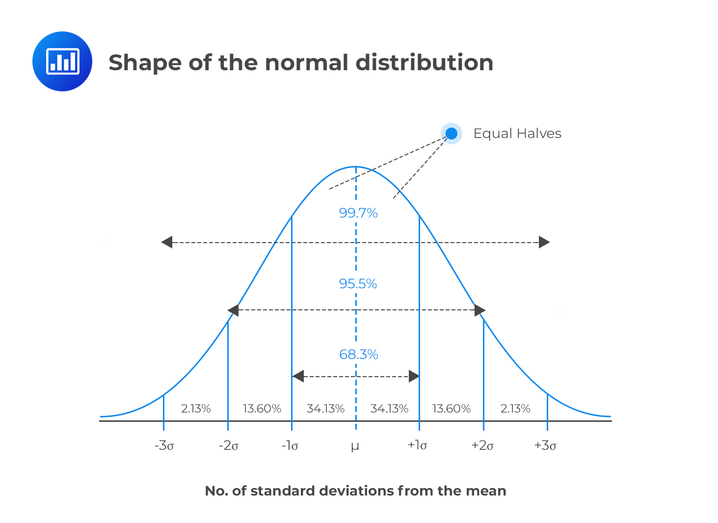
• All normal distributions can be described by their mean and their standard deviation

• This one is called “sampling distribution of the sample mean”

  • Centered around our estimate \(\hat{p}\)
  • \(SE = \sqrt{\frac{Var (Support)}{n}}\)

• Knowing it is a normal distribution helps us quantify the uncertainty in our estimates

Standard Errors

Confidence Intervals

Confidence Intervals

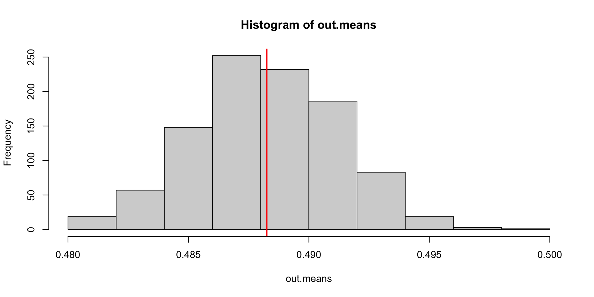
• Because of the properties of the normal distribution, we know that 95% of the density will be within the following range:

Computing CI’s: Example

# standard deviation of the sampling distribution computed with the formula
se <- round(sqrt(var(brex$exit, na.rm = T)/nrow(brex)),3)
# An analytic solution to the confidence interval
(ci_95 <- c(phat - (1.96*se), phat + (1.96*se)))

[1] 0.4823528 0.4941128

# We can check that it's the same as the interval that leave 95% of the mass inside
# of the sampling distribution 
quantile(out.means, c(.025, .975))

     2.5%     97.5% 
0.4824196 0.4939738 

Linear Regression

• We can think of the parameters of a linear regression in the same way.

• \(\alpha\) an intercept, common to all units.

• \(\beta\) the slope, common to all units.

• We need to describe the relationship between X and Y with a line using information from our sample

Linear Regression: Intuition

• Our data includes the outcome \(y_i\) and our explanatory variable \(x_i\)

• But we can draw infinite lines through those points

• How to choose the correct \(\widehat{\beta}\) and \(\widehat{\alpha}\), like we chose the correct \(\widehat{p}\)?

Linear Regression: Intuition

• If we have a slope and an intercept, for every \(X_i\), the equation of a line gives us a predicted \(Y_i\), or \(\widehat{Y_i}\)

• So, for each plausible estimates of \(\widehat{\beta}\) and \(\widehat{\alpha}\) we can calculate the prediction error

\[\begin{align*} \hat{\varepsilon}_i =& Y_i - \hat{Y_i} \\ \hat{\varepsilon}_i =& Y_i - \hat{\alpha} - \hat{\beta} x_i \end{align*}\]

Linear Regression: Intuition

• If we add up the prediction error for each observation, we get the Sum of Squared Residuals

\[\begin{equation*} SSR = \widehat{\varepsilon}^2 = (Y_i - \widehat{\alpha} - \widehat{\beta}X_i)^2 \end{equation*}\]

• Minimizing this objective yields the “ordinary least squares” (OLS) estimates of \(\alpha\) and \(\beta\)

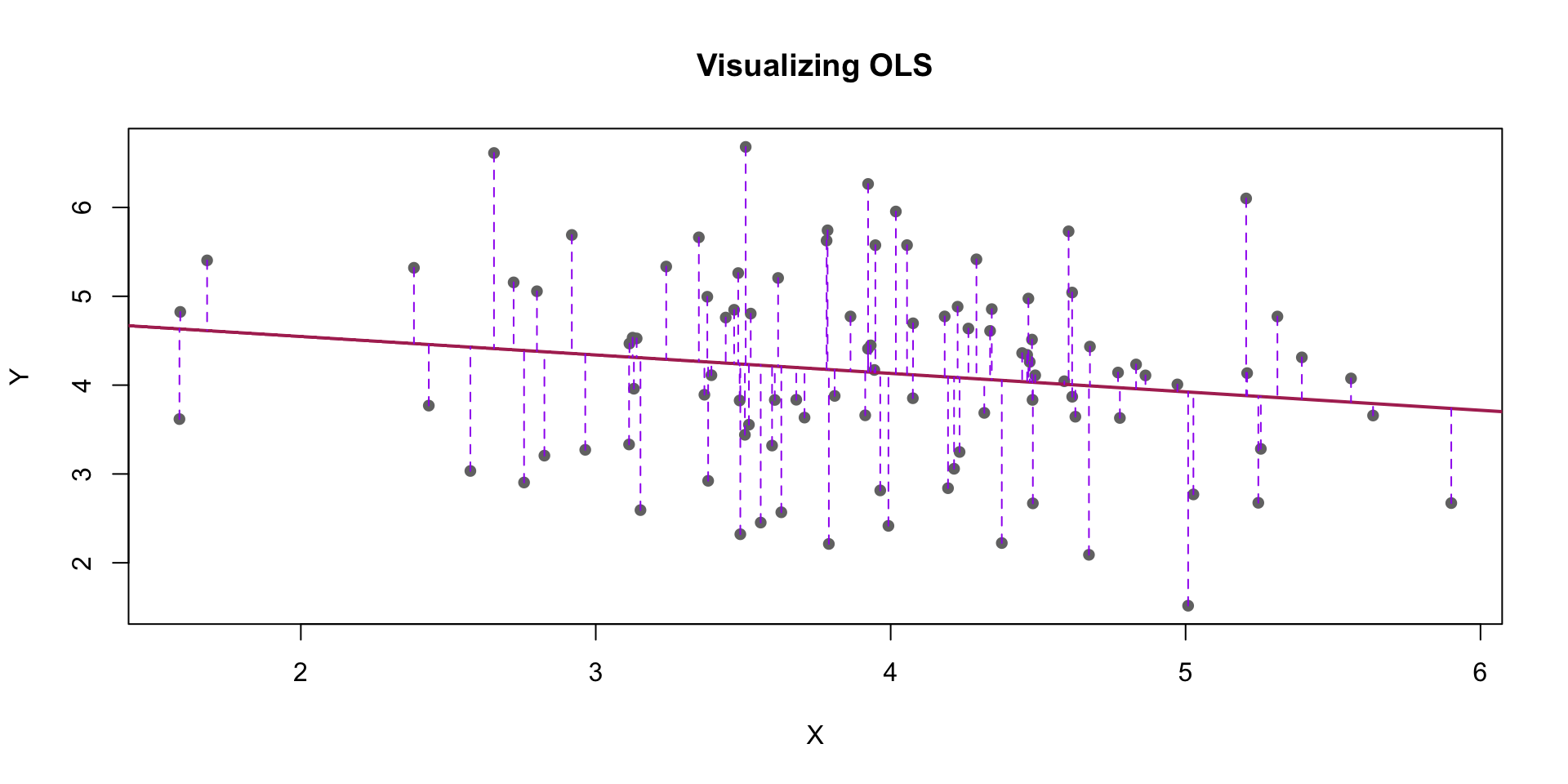
Linear Regression: Simulation

# Simulated data
set.seed(8)
# TRUE alpha and beta
alpha <- 5
beta <- -.216
x <- rnorm(100, 4, .8) # 
error <- rnorm(100, 0, 1)
# relationship is linear by construction because I'm simulation god!!
y <- alpha + (beta*x) + error

Linear Regression: Simulation

# Fit linear model
model <- lm(y ~ x)
# Predict $y_hat$ or the expected y given the model and x
y_pred <- predict(model)
# Plot the data
plot(x, y, main="Visualizing OLS", xlab="X", ylab="Y", pch=16, col="gray45")
# Add best fit line
abline(model, col="maroon", lwd=2)
# Draw vertical lines showing each prediction error
segments(x, y, x, y_pred, col="purple", lty=2)

Linear Regression: Interpretation

• Why are \(\hat{\beta}\) and \(\hat{\alpha}\) different from \(\alpha\) and \(\beta\)?

Call:
lm(formula = y ~ x)

Residuals:
    Min      1Q  Median      3Q     Max 
-2.4061 -0.8055  0.1533  0.6918  2.4457 

Coefficients:
            Estimate Std. Error t value Pr(>|t|)    
(Intercept)   4.9658     0.5027   9.879   <2e-16 ***
x            -0.2082     0.1251  -1.664   0.0993 .  
---
Signif. codes:  0 '***' 0.001 '**' 0.01 '*' 0.05 '.' 0.1 ' ' 1

Residual standard error: 1.074 on 98 degrees of freedom
Multiple R-squared:  0.02748,   Adjusted R-squared:  0.01755 
F-statistic: 2.769 on 1 and 98 DF,  p-value: 0.09932

         x 
-0.2081563 

[1] 0.1250993

Linear Regression

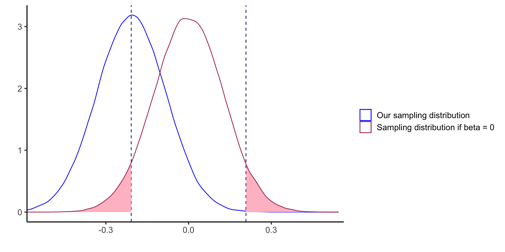
• Estimates of \(\hat{\beta}\) and \(\hat{\alpha}\) have uncertainty

Hypothesis Testing and P-values

• We are often interested in determining whether the true parameter is different from zero with a pre-specified level of confidence

• We are going to reject \(H_0\) in favor of \(H_1\) if we are sufficiently confident we aren’t making a (type I) mistake

P-value

1. Assume the true effect/parameter is 0

2. “Draw” the sampling distribution of the parameter

   • Remember we know that its sd = se

3. Calculate the probability of observing an estimate at least as extreme as the one you observed with your sample if the true parameter is zero

4. If you are doing a two-tailed test, use absolute value

P-value

• Simulated data to visualize the p-value

Statistical Significance

• If you are using a level of statistical significance of 95%, you reject \(H0: \beta = 0\) if \(\text{p-value} \leq .05\)

• If you are using a level of statistical significance of 99%, you reject \(H0: \beta = 0\) if \(\text{p-value} \leq .01\)

• When we have estimates with a p-value less or equal to that, we say our coefficient is “statistically significant”

• It just means we are sure enough the parameter is different from zero

• In papers, they report this with different number of stars!

Statistical Significance

• In our example, would we reject \(H0: \beta = 0\) with 90% confidence? With 95% confidence? With 99%?

summary(model)

Call:
lm(formula = y ~ x)

Residuals:
    Min      1Q  Median      3Q     Max 
-2.4061 -0.8055  0.1533  0.6918  2.4457 

Coefficients:
            Estimate Std. Error t value Pr(>|t|)    
(Intercept)   4.9658     0.5027   9.879   <2e-16 ***
x            -0.2082     0.1251  -1.664   0.0993 .  
---
Signif. codes:  0 '***' 0.001 '**' 0.01 '*' 0.05 '.' 0.1 ' ' 1

Residual standard error: 1.074 on 98 degrees of freedom
Multiple R-squared:  0.02748,   Adjusted R-squared:  0.01755 
F-statistic: 2.769 on 1 and 98 DF,  p-value: 0.09932

Summing Up: 2 Takeaways

• The representative-ness of our samples is crucial to make inferences abt. population

  • The more observations we have, the better “powered” we are to detect small effects

  • But sample size does not substitute for representative-ness

• Statistical significance is important but it is NOT a measure of SCIENTIFIC importance

  • Statistical significance just means an effect or difference is likely NOT to be zero