Migration 1

Plus Difference-in-Differences

Author

Affiliation

Jeremy Springman

University of Pennsylvania

Logistics

Assignments

• Today
  • Rozo and Grossman (2025) (download the pdf and/or watch the YouTube video)
  • Gazeaud, Jules, Eric Mvukiyehe, and Olivier Sterck (2020)
  • Sviatschi (2022)

Agenda

1. Research Design Debrief
2. Migration
3. Causal Inference with Observational Data: Difference-in-Differences

Research Design Debrief

Debrief

Submissions

• You need to check what you send me…
• Read the basic instructions (quarto + html file)
• I didn’t penalize anyone, but next time I will

Research Designs

• Justify your sample
• Just “controlling for observables” will not get you full credit
• Next week, we’ll cover essentials… bring your questions!

Migration Overview

Overview of International Migration

Economic Equilibrium

• Push factors
• Pull factors
• Costs

Economic Equilibrium: Push

Push factors: origin country factors that affect the well-being

• Demographics: youth bulge
• Living standards: poor infrastructure, crime
• Economic opportunities: unemployment
• Politics: exclusion

Economic Equilibrium: Pull

Pull factors: destination country factors that affect expected well-being

• Demographics: aging population
• Living standards: good infrastructure, security
• Economic opportunities: labor demand, credit
• Politics: inclusion

Economic Equilibrium: Costs

Costs: factors that shape the costs of migrating

• Legal restrictions
• Transportation
• Asset mobility

Economic Equilibrium Perspective

• Migration decisions are based on expected return
• Movements from poorer to richer regions will equalize wages

Migration Systems

Macro linkages between sending and receiving countries

• Migration is driven by prior links between sending and receiving countries
  • Colonization, political or cultural influence, trade, language

Micro linkages between households

• Migration is driven by prior links between individuals and households
  • Social ties to households in the destination country

Rozo & Grossman

Quiz

5 minutes: send me a Slack DM with something you learned from this article

Trends: Displacement

Trends: Displacement

Trends: Conflict

• War deaths continue to decline
• Interstate wars are rare by historical standards
• Geopolitical tensions are increasing
• Number, intensity, complexity, and duration of civil wars are increasing

Trends: Conflict

Trends: Climate

• 78% of global land area has become drier over the past 30 years
• Warmer temperatures are causing extreme weather events

Trends: Research

Trends: Research

Impact on Host: Labor markets

• Who gets hurt?
• Who benefits?
• Net effects effects?
  • Short-term challenges
  • Long-term growth

Benefit: skilled laborers, formal businesses Hurt: unskilled (women, youth), informal businesses

Impact on Host: Other

• Service provision
  • Displacement effects (public to private)
  • Disease burden
• Politics
  • Wealth
  • Prior exposure

Supporting Migrants

Unique challenges for forced migrants?

• Loss of assets
• Trauma and mental health
• Legal uncertainty
• Language and cultural barriers

Supporting Migrants

Cash transfers

• Short-term increases in consumption, well-being

Labor market integration

• Increased consumption, well-being
• Reduced crime, fertility
• Kakuma vs Kalobeyei; Uganda business mentors

Supporting Migrants

• Mental health
• Social cohesion
  • Teacher bias
  • Shared aid + integration policies
  • Perspective-taking, contact

Policy Implications

• Shift from humanitarian response to self-reliance
• Allow hosts to benefit from aid
• Increase labor market integration
• Address discrimination and mental health

Gazeaud et al. (2023)

Constraints to migration

• Migration causes huge income gains
• Desire for migration is extremely high
• Actual migration flows are relatively small
• Why?

Intervention

Conditional cash transfer

• Cash payment for labor on public works

Mechanisms:

1. Liquidity
2. Opportunity cost
3. Collateral and access to credit
4. Risk-aversion

Findings

• Treatment households 38% more likely to migrate
• How did they measure spillovers?
• Mechanisms:
  • What were the mechanisms at play?
  • How did they reach these conclusions?

Findings

Policy Implications

How does this relate to the equilibrium model?

Policy implications

• The poorest individuals in sending countries are not the most likely to migrate (Clements and Mendola, 2020)
• Improving welfare in sending countries will not necessarily reduce desire to migrate
• Networks may be less influential (over short time periods and with large pre-treatment migration)

Difference-in Differences

Review

• What is an interaction term?
• What are fixed effects?
• Why do we like randomization?

Identification strategy

In the real world, there are always confounders that we can’t observe (measure) or adjust for

• A research design that allows us to isolate a causal effect from observational data
• Approximates an experiment by ensuring that the treatment and untreated (control) group are similar
• These strategies rely on assumptions that we can attempt to validate

Holy Trinity of Causal Inference

1. Difference-in-Differences
2. Regression Discontinuity
3. Instrumental Variables

Difference-in-Differences

\[ Y_{it} = \alpha + \beta_1 \text{Treatment}_i + \beta_2 \text{Post}_t + \gamma (\text{Treatment}_i \times \text{Post}_t) + \epsilon_{it} \]

• \(\gamma (\text{Treatment}_i \times \text{Post}_t)\)
• Assumes measurement at two points in time

Simulation Example

# Load required libraries
library(dplyr)
library(modelsummary)

# Generate example data
set.seed(123)
data <- data.frame(
  treatment = rep(c(1, 0), each = 100),
  post = rep(c(1, 0), each = 50, times = 2),
  outcome = c(rnorm(50, mean = 10, sd = 4), # control: pre-treatment
              rnorm(50, mean = 10, sd = 4), # control: post-treatment
              rnorm(50, mean = 10, sd = 4), # treatment: pre-treatment
              rnorm(50, mean = 12, sd = 4)) # treatment: post-treatment
)

head(data)

  treatment post   outcome
1         1    1  7.758097
2         1    1  9.079290
3         1    1 16.234833
4         1    1 10.282034
5         1    1 10.517151
6         1    1 16.860260

Simulation Example

# Summarize the output
modelsummary(
  list(lm(outcome ~ treatment + post, data = data),# standard model
       lm(outcome ~ treatment * post, data = data)), # difference-in-differences model
  estimate  = "{estimate}{stars} ({std.error})",
             statistic = NULL,
  gof_omit = 'IC|RMSE|Log|F|R2$|Std.')

	Model 1	Model 2
(Intercept)	11.475*** (0.466)	12.155*** (0.531)
treatment	−0.208 (0.538)	−1.570* (0.751)
post	−1.809*** (0.538)	−3.171*** (0.751)
treatment × post		2.723* (1.062)
Num.Obs.	200	200
R2 Adj.	0.045	0.072

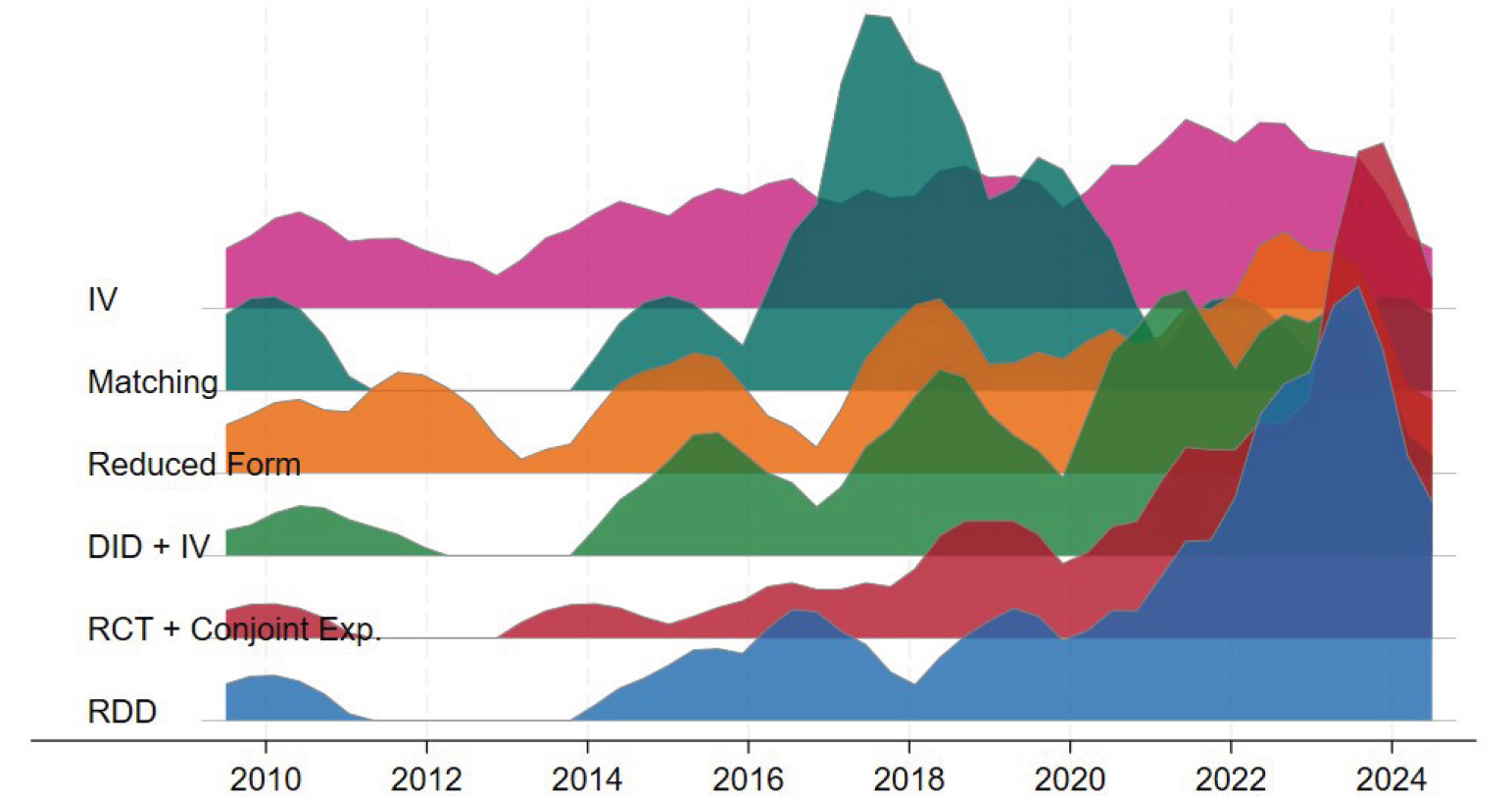
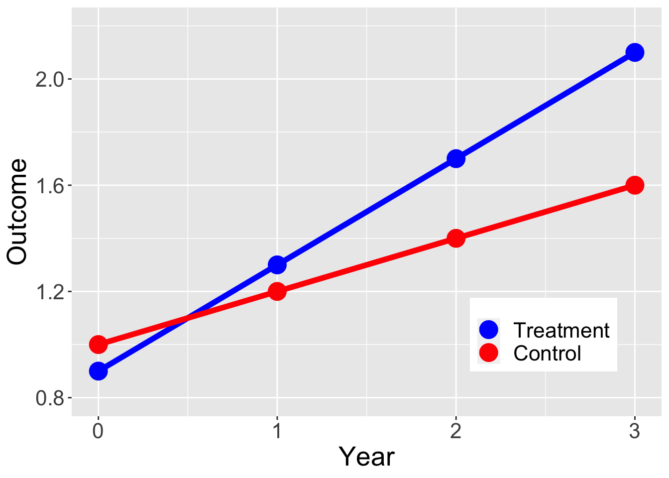
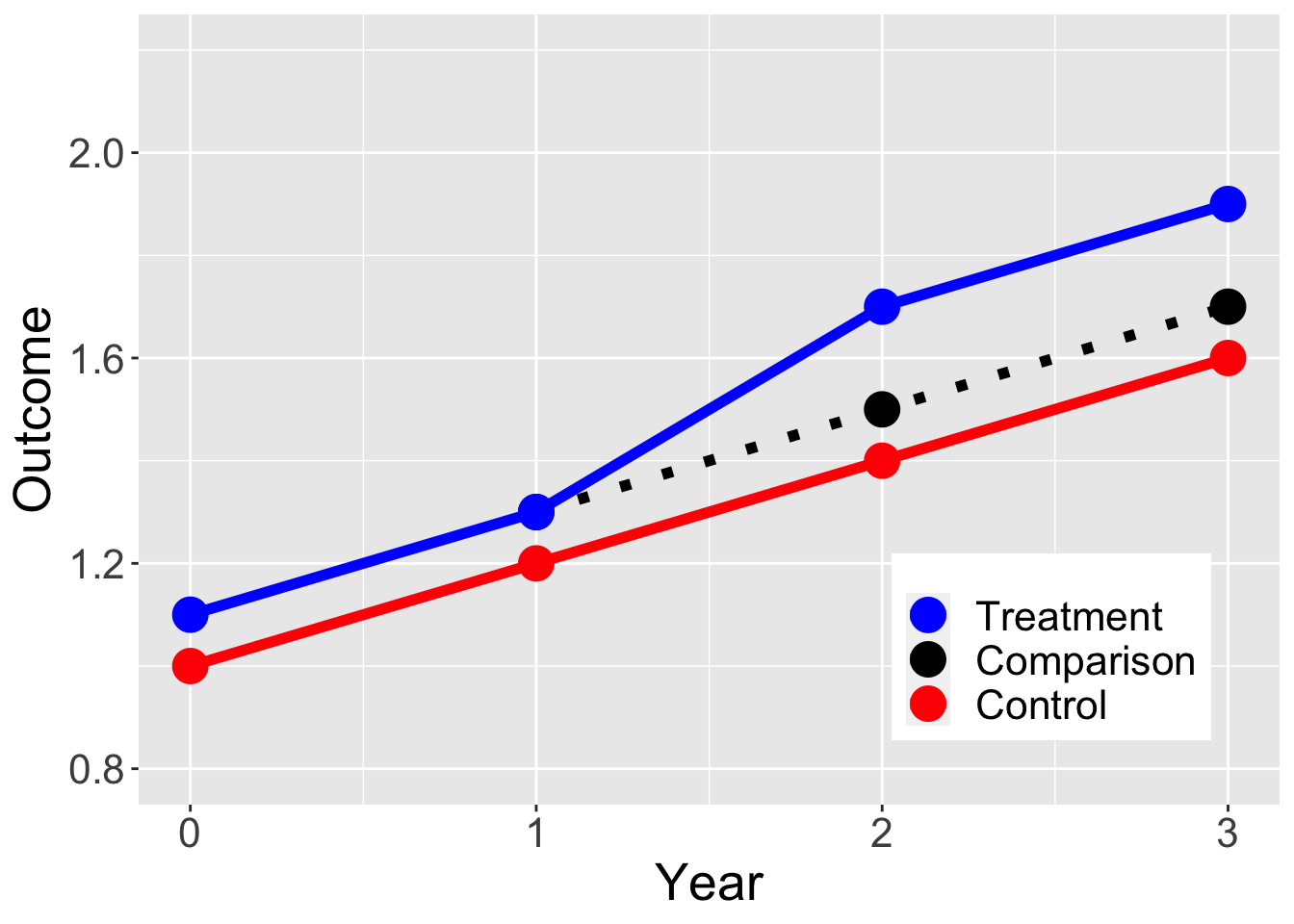
DiD: Assumptions

• Treatment and control units would have changed in similar ways
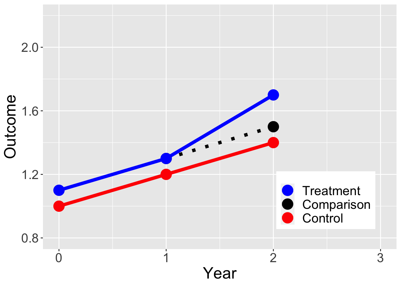
  • Parallel trends
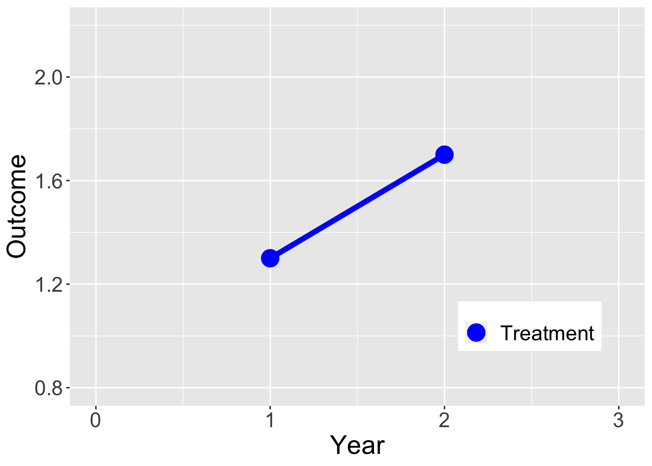
• Requires at least 3 observation periods

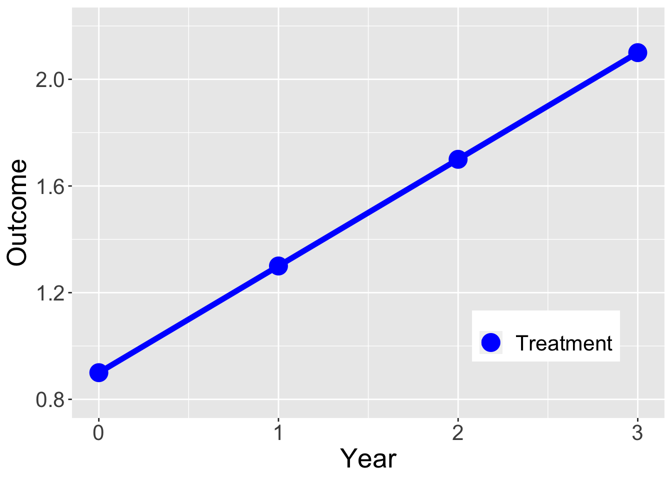
Why can’t we just observe how units change over time?

library(ggplot2)

Year = c(0,1,2,3)
Outcome = c(NA, 1.3, 1.7, NA)
Treatment = c("Treatment", "Treatment","Treatment","Treatment")

dat = data.frame(Year, Outcome, Treatment)

ggplot(data = dat, aes(x = Year, y = Outcome, group = Treatment, color = Treatment)) +
  geom_line(aes(linetype=Treatment),size=2) +
  geom_point(size = 6) +
  xlim(0,3) + 
  ylim(0.8, 2.2) +
  scale_linetype_manual(values=c("solid", "solid")) +
  scale_color_manual(values = c("blue") ) +
  theme(legend.position = c(0.8, 0.2), text = element_text(size=20),
        legend.title=element_blank())

Why can’t we just observe how units change over time?

Year = c(0,1,2,3)
Outcome = c(0.9, 1.3, 1.7, 2.1)
Treatment = c("Treatment", "Treatment","Treatment","Treatment")

dat = data.frame(Year, Outcome, Treatment)

ggplot(data = dat, aes(x = Year, y = Outcome, group = Treatment, color = Treatment)) +
  geom_line(aes(linetype=Treatment),size=2) +
  geom_point(size = 6) +
  xlim(0,3) + 
  ylim(0.8, 2.2) +
  scale_linetype_manual(values=c("solid", "solid")) +
  scale_color_manual(values = c("blue") ) +
  theme(legend.position = c(0.8, 0.2), text = element_text(size=20),
        legend.title=element_blank())

Why can’t we just compare units without randomization?

Year = c(0,1,2,3)
Outcome = c(NA, 1.2, 1.4, NA, 
            NA, 1.3, 1.7, NA)
Treatment = c("Control", "Control","Control","Control", 
              "Treatment", "Treatment", "Treatment", "Treatment")

dat = data.frame(Year, Outcome, Treatment)
dat$Treatment = factor(dat$Treatment, levels = c("Treatment", "Control"))

ggplot(data = dat, aes(x = Year, y = Outcome, group = Treatment, color = Treatment)) +
  geom_line(aes(linetype=Treatment),size=2) +
  geom_point(size = 6) +
  xlim(0,3) + 
  ylim(0.8, 2.2) +
  scale_linetype_manual(values=c("solid", "solid")) +
  scale_color_manual(values = c("blue", "red") ) +
  theme(legend.position = c(0.8, 0.2), text = element_text(size=20),
        legend.title=element_blank())

Why can’t we just compare units without randomization?

Year = c(0,1,2,3)
Outcome = c(1, 1.2, 1.4, 1.6, 
            0.9, 1.3, 1.7, 2.1)
Treatment = c("Control", "Control","Control","Control", 
              "Treatment", "Treatment", "Treatment", "Treatment")

dat = data.frame(Year, Outcome, Treatment)
dat$Treatment = factor(dat$Treatment, levels = c("Treatment", "Control"))


ggplot(data = dat, aes(x = Year, y = Outcome, group = Treatment, color = Treatment)) +
  geom_line(aes(linetype=Treatment),size=2) +
  geom_point(size = 6) +
  xlim(0,3) + 
  ylim(0.8, 2.2) +
  scale_linetype_manual(values=c("solid", "solid")) +
  scale_color_manual(values = c("blue", "red") ) +
  theme(legend.position = c(0.8, 0.2), text = element_text(size=20),
        legend.title=element_blank())

Why can’t we just compare units without randomization?

Year = c(0,1,2,3)
Outcome = c(NA, 1.3, 1.5, NA,
            1, 1.2, 1.4, NA,
            1.1, 1.3, 1.7, NA)
Treatment = c("Comparison","Comparison","Comparison","Comparison",
              "Control", "Control","Control","Control",
              "Treatment", "Treatment", "Treatment", "Treatment")

dat = data.frame(Year, Outcome, Treatment)
dat$Treatment = factor(dat$Treatment, levels = c("Treatment", "Comparison", "Control"))

ggplot(data = dat, aes(x = Year, y = Outcome,  color = Treatment)) +
  geom_line(aes(linetype=Treatment),size=2) +
  geom_point(size = 6) +
  ylim(0.8, 2.2) +
  scale_linetype_manual(values=c("solid", "dotted", "solid")) +
  scale_color_manual(values = c("blue", "black", "red"  ) ) +
  theme(legend.position = c(0.8, 0.2), text = element_text(size=20),
        legend.title=element_blank())

Why can’t we just compare units without randomization?

Year = c(0,1,2,3)
Outcome = c(NA, 1.3, 1.5, 1.7,
            1, 1.2, 1.4,1.6,
            1.1, 1.3, 1.7, 1.9)
Treatment = c("Comparison","Comparison","Comparison","Comparison",
              "Control", "Control","Control","Control",
              "Treatment", "Treatment", "Treatment", "Treatment")

dat = data.frame(Year, Outcome, Treatment)
dat$Treatment = factor(dat$Treatment, levels = c("Treatment", "Comparison", "Control"))

ggplot(data = dat, aes(x = Year, y = Outcome,  color = Treatment)) +
  geom_line(aes(linetype=Treatment),size=2) +
  geom_point(size = 6) +
  ylim(0.8, 2.2) +
  scale_linetype_manual(values=c("solid", "dotted", "solid")) +
  scale_color_manual(values = c("blue", "black", "red"  ) ) +
  theme(legend.position = c(0.8, 0.2), text = element_text(size=20),
        legend.title=element_blank())

Sviatschi (2022)

Sviatschi (2022)

• What is the effect of mass deportations on the root causes of migration?

Three sources of variation

1. Geography (birth municipality)
2. Time (policy change)
3. Age (recruitment age)

Identifying assumption

• Municipalities where gang-deportees were born would have changed in similar ways to other municipalities in the absence of a policy change

Findings

Policy Implications

• Addressing pull factors can have unintended affects on push factors in complex ways

Threats to Inference

• Confounders
• Colliders
• Mechanisms
• Reverse Causality

Adjusting on Observables

• Matching
• Weighting
• Synthetic Control (very fancy weighting)

Validity

• Internal validity
• External validity
• What are the trade-offs between experiments and observational studies?
  • Experiments have more internal validity
  • But… they often have synthetic treatments, convenience samples
• Where are these studies used in the real-world?

3ie Evidence Review

Irregular Migration Evidence Review

Objective:

• Review evidence efficacy of interventions designed to target the root causes of irregular migration

Root causes: social and political conditions that induce departures

1. Lack of economic opportunity
2. Lack of capacity to adopt to shocks
3. High levels of violence
4. Lack of regular migration channels

Irregular Migration Evidence Review

What is irregular migration?

• Migration outside legal channels

Why is it different from regular migration?

• Additional risks relative to legal migration (violence, exploitation, access to legal system)

Findings

Studies reporting migration outcomes are concentrated on 3 intervention categories:

1. Human capital strengthening
2. Active labor market policies
3. Information campaigns

Conclusions

• Some evidence on interventions that address the root causes of irregular migration
• Almost no evidence looking at irregular migration as a primary outcome
• A number of studies are ongoing